【R】最短ドライブ距離の計算

ドライブで最短距離で移動したいことは、多々ありますよね。今は、カーナビがあるので、その最短距離の探索なんてする必要がないのですが、PC画面上で見たいときもあります。Googleを使えば一発なんですが、データとして扱うには、また別の方法が必要です。

で、今回は、　”R”　を使ってみます。

こちらを参考に表題を実施しました。

library(dodgr)
class (hampi)
#> [1] "sf"         "data.frame"
dim (hampi)
#> [1] 203  15
graph <- weight_streetnet (hampi, wt_profile = "foot")
class (graph)
#> [1] "data.frame"      "dodgr_streetnet"
dim (graph)
#> [1] 5973   15
head(graph)
  
library(tidyverse, quietly=T) # data processing
library(osmdata, quietly=T) # load osm data
library(sf, quietly=T) # use spatial vector data 
library(dodgr, quietly=T) # driving distance
library(geosphere, quietly=T) # aerial distance
library(classInt, quietly=T) # legend
library(extrafont, quietly=T) # font
set.seed(20210618)
#download official 2021 Serbian census circles
u <- "https://github.com/justinelliotmeyers/Official_Serbia_2021_Administrative_Boundaries/raw/main/popisni_krug-gpkg.zip"
download.file(u, basename(u), mode="wb")
unzip("popisni_krug-gpkg.zip")
#load census circles
pk <- st_read(paste0(getwd(), "/tmp/data/ready/pk/", "popisni_krug.gpkg"), stringsAsFactors = FALSE) %>% 
  st_transform(4326) %>% 
  st_as_sf()
# define Belgrade's bounding box based on ggmap's bounding box
bg_map <- ggmap::get_map(getbb("Belgrade"), 
                         maptype = "toner-lite", 
                         source = "stamen", 
                         color="bw", 
                         force=T)
bg_bbox <- attr(bg_map, 'bb')
bbox <- c(xmin=bg_bbox[,2], 
          ymin= bg_bbox[,1], 
          xmax= bg_bbox[,4],
          ymax=bg_bbox[,3])
#filter Belgrade
pkb <- st_crop(pk, bbox)
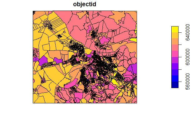
plot(pkb["objectid"])

こんな風に結果を出力できます。